Chapter 3, Section 3.3

Treatment of Lead Exposed Children Trial (TLC)

Time Plots of Blood Lead Levels 

. use "tlc.dta"

. reshape long y, i(id) j(time)

(note: j = 0 1 4 6)

Data                               wide   ->   long

-----------------------------------------------------------------------------

Number of obs.                      100   ->     400

Number of variables                   6   ->       4

j variable (4 values)                     ->   time

xij variables:

                           y0 y1 ... y6   ->   y

-----------------------------------------------------------------------------

. tsset id time

panel variable:  id (strongly balanced)

time variable:  time, 0 to 6, but with gaps

delta:  1 unit

. label variable y "Blood Lead Level (mcg/dL)"

. label variable time "Time (in weeks)"

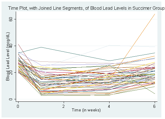
. xtline y, overlay legend(off) ///

t1("Time Plot, with Joined Line Segments, of Blood Lead Levels in Succimer Group")

. ssc install xtgraph

checking xtgraph consistency and verifying not already installed...

installing into c:\ado\plus\...

installation complete.

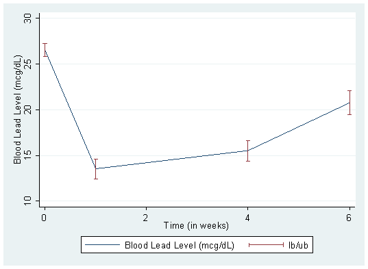
. xtgraph y if (trt==1), av(mean) bar(se)

Six Cities Study of Air Pollution and Health

Time Plots of Log(FEV1/Height) 

. use "fev.dta"

. drop if (id==197)

(1 observation deleted)

. gen y = logfev1 - log( ht)

. label variable y "Log(FEV1/Height)"

. label variable age "Age (in years)"

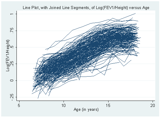
. graph twoway (scatter y age, ylabel(-0.25 0 to 1.0) msym(i) connect(L) ///  

t2("Line Plot, with Joined Line Segments, of Log(FEV1/Height) versus Age"))

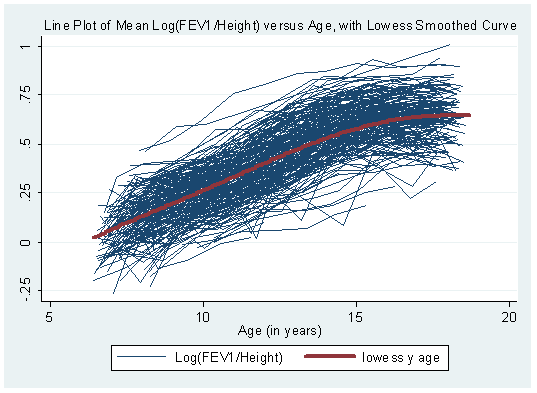
. graph twoway (scatter y age, ylabel(-0.25 0 to 1.0) msym(i) connect(L)) ///

     (lowess y age, lwidth(thick) ///

t2("Line Plot of Mean Log(FEV1/Height) versus Age, with Lowess Smoothed Curve"))